Graph Iterated Function Systems: Adding Structure to Self-Similarity
Provides a mathematical bridge from fractal geometry to hierarchical time series and the embedding spaces that AI models and transformers operate on.
How a directed graph can enable richer fractals, with different patterns in different parts, while providing a basis for AI embedding vectors.
This article series establishes the mathematical foundations for representing time series as self-similar hierarchical structures, with a framework that underpins a novel AI architecture for temporal data. It refines the concepts outlined in the previous article on Iterated Function Systems (IFS) to introduce the concept of a directed graph that controls which parts relate to which, making self-similarity expressive enough to model real-world hierarchical decompositions as the basis of an embedding space for AI models.
Previously: Iterated Function Systems · Next: Temporal Embeddings
In the previous article, we saw how a standard IFS works: take a handful of contraction mappings, apply them over and over, and a fractal appears. The Cantor set, the Sierpinski triangle, the Barnsley fern[1], all produced by iterating a fixed set of shrinking functions.
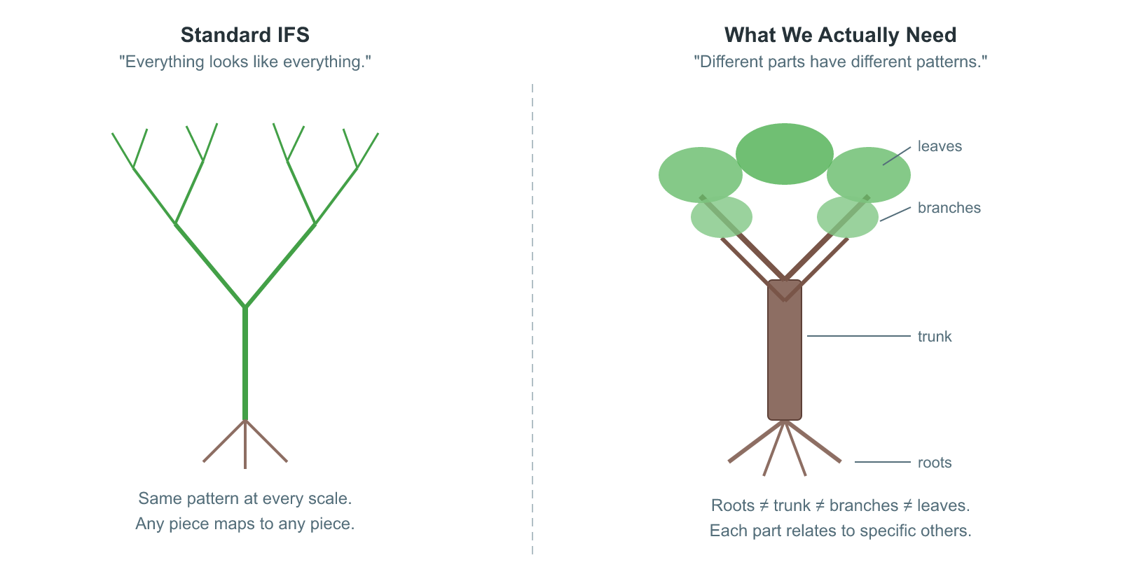
But there's a limitation hiding in that simplicity. In a standard IFS, every function is applied at every iteration, and there's no rule saying which functions can act on which parts. The result is uniform self-similarity: every part of the fractal looks like every other part. That's fine for the Sierpinski triangle, where the three corners are genuinely identical. But what about structures where different regions have different patterns?
Think of a tree. The roots, the trunk, the branches, and the leaves all have self-similar structure, but they don't all look the same. A branch splits into smaller branches, not into roots. A leaf's veins branch in a pattern distinct from the trunk's bark. The self-similarity is directed: specific parts relate to specific other parts, and the relationships follow a structure.
A Graph Iterated Function System (GIFS) captures exactly this. Instead of a flat list of functions, a GIFS organizes them as edges in a directed graph. The graph controls which transformations can compose: a function on edge $(i, j)$ decomposes vertex $i$'s component into a smaller piece that becomes part of vertex $j$'s component. Different vertices can have different roles, different numbers of incoming edges, and different relationships to the rest of the system. The result is a family of related shapes, each one defined by its position in the graph, rather than a single monolithic fractal.
This is the bridge between the elegant theory of IFS and the messy, structured reality of hierarchical data and time series data in particular. As we will see later in this article, GIFS provides a natural basis for embedding vectors that can be used with novel AI transformer architectures.
From IFS to GIFS: What Changes?
Before diving into definitions, it's worth understanding the shift in thinking. In a standard IFS, you have one shape and $N$ functions that all act on that same shape. The attractor is a single compact set. Everything is symmetric: function $w_1$ has no special relationship to $w_2$, and any function can follow any other in the iteration.
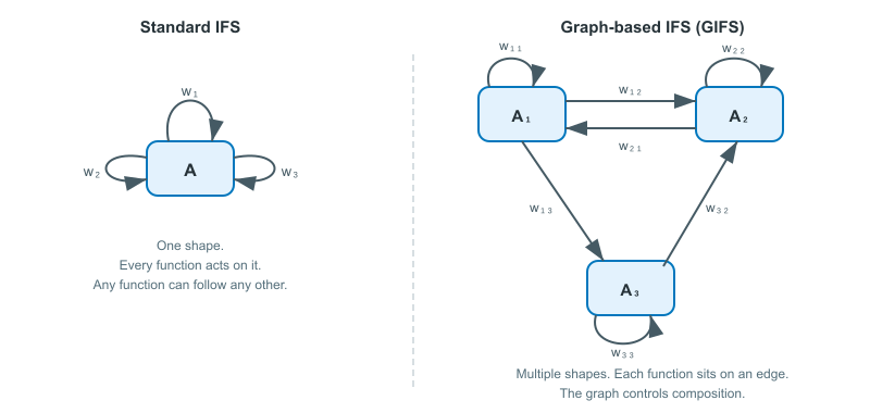
A GIFS changes this in a specific way. Instead of one shape, you have $n$ shapes, one for each vertex in a directed graph. Instead of a flat list of functions, each function sits on an edge of the graph and maps from one vertex's shape to another's. The graph structure dictates which compositions are allowed.
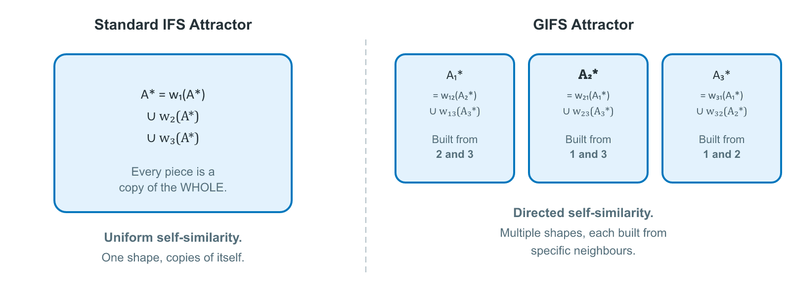
Here's the key intuition: in a standard IFS, the attractor equation says "the whole is the union of shrunken copies of the whole." In a GIFS, each vertex's attractor says "I am the union of shrunken copies of my neighbours' attractors, as determined by the edges pointing out from me." Each component is built from pieces of other components, and the graph says which pieces go where.
This might sound like a small change, but what it does to self-similarity is fundamental.
In a standard IFS, self-similarity is literal and total: every piece of the attractor is a miniature copy of the entire attractor. Zoom into any region of the Sierpinski triangle and you find smaller Sierpinski triangles. Zoom into those and you find even smaller ones. The whole is always present in every part. There is only one shape in the system, so the only thing any part can resemble is that shape.
A GIFS breaks this. When you zoom into a piece of component $A_i$, you don't necessarily find a smaller copy of $A_i$. You find a shrunken copy of whichever neighbouring components $A_j$ that the relevant graph edge points to. $A_j$ might look completely different from $A_i$. Zoom into that piece and you find copies of whatever components $A_j$'s edges point to, and so on. What you see at each level of magnification depends on the path you're following through the graph.
Self-similarity still exists, but it's no longer a relationship between a shape and itself. It's a relationship between shapes, mediated by the graph. A piece of one component resembles a different component, which in turn contains pieces resembling yet other components, and the graph determines the entire chain. Mathematicians call this graph-directed self-similarity. A standard IFS's "every part looks like the whole" is just the special case where the graph has a single vertex, so there's only one shape anything can resemble.
This is what makes different parts of the system genuinely different. The topology of the graph controls which structures appear where, and the result can be far richer than anything uniform self-similarity can produce.
Definition
A GIFS has two ingredients. The first is a directed graph whose vertices represent the different component types in the system and whose edges represent the transformations between them. Each edge says: this component can contribute a shrunken piece of itself to that component. The direction matters. An edge from vertex A to vertex B doesn't imply an edge from B back to A.
The second ingredient is a contraction mapping sitting on each edge. This is a specific shrinking function that says exactly how one component's shape gets transformed into a piece of another's. Every edge carries its own contraction, so different relationships can shrink by different amounts or in different ways.
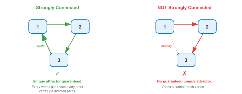
In the classical literature, the graph is assumed to be strongly connected, meaning every vertex can reach every other through some chain of edges. This ensures all components are genuinely interdependent and is required for the deeper results on Hausdorff dimension. However, the attractor, which is the central object of interest, exists for any contractive system, strongly connected or not.
Following Barnsley and Vince[2] and Edgar[3], the formal definition of a Graph Iterated Function System is:
- A finite directed graph $G = (V, E)$ with vertex set $V = [n] = {1, 2, \ldots, n}$. For each edge $e \in E$, the tail $e^-$ is its source vertex and the head $e^+$ is its target vertex. We write $E_i$ for the set of edges with tail $i$.
- A set of invertible contraction mappings $\mathbf{F} = {f_e : e \in E}$, where each $f_e: \mathbb{R}^d \to \mathbb{R}^d$ is contractive. In the classical literature, contractivity is defined pointwise: $|f_e(x) - f_e(y)| \leq \lambda_e \cdot |x - y|$ for all $x, y$, with contraction factor $\lambda_e < 1$. This is the condition required for the Banach fixed-point argument and the Hausdorff dimension formula. For the rooted variant introduced below, a weaker condition (that each edge mapping strictly reduces the bounding region), as we discuss in the section on the rooted GIFS.
The GIFS is the pair $(G, \mathbf{F})$.
We also consider a rooted variant below where the graph is a tree. The vertices are the "types" or "roles" or "shapes" in the system. The edges are the transformations. The graph controls which compositions are permitted.
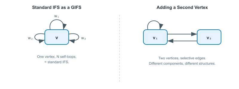
Notice how this generalizes standard IFS. A standard IFS is just a GIFS with a single vertex and $N$ self-loops. Every function maps from the one component back to itself, and every function can follow every other, because there's only one vertex. The moment you add a second vertex, you gain the ability to have different components with different structures.
Rooted GIFS
A standard GIFS treats all vertices as peers in a strongly connected graph. Every component depends on every other, and there is no preferred starting point. But many real-world structures have an inherent top: a whole that decomposes into parts, which decompose into smaller parts, down to some finest level. A time series has an overall shape that breaks into segments, which break into sub-segments, and so on. This calls for a rooted variant of the GIFS where the graph fans out from a single starting vertex.
Barnsley and Vince[2:1] introduce a related concept: the pre-tree, a set of directed paths through a GIFS graph that all begin at the same vertex $r$, called the root, and fan outward toward leaf vertices. Their Proposition 1 shows that every pre-tree generates a unique rooted directed tree via a graph homomorphism. The pre-tree captures the hierarchical decomposition of the root vertex's attractor, how it breaks into pieces, how those pieces break into sub-pieces, and so on through successive levels. But in their formulation, the pre-tree is a structure built on top of a general GIFS graph; the graph itself remains strongly connected.
For hierarchical applications, we go further and make the tree structure part of the definition itself. A rooted GIFS is a triple $(G, \mathbf{F}, r)$ where:
- $G = (V, E)$ is a finite directed graph with vertex set $V = [n]$ and a distinguished root vertex $r \in V$.
- The non-self-loop edges of $G$ form a rooted directed tree at $r$, with every such edge directed away from the root (from parent to child). For every vertex $v \in V$, there is a unique directed path from $r$ to $v$.
- Leaf vertices (vertices with no outgoing edges) carry no edges in $E$. Their attractors are not computed from contractions. They are given directly as input data. In our application, a segmentation algorithm decomposes the raw time series into non-overlapping segments, and each segment becomes a leaf vertex in the tree. The contraction mappings on the internal edges are then fitted to describe how each parent segment relates to its children. The construction of this tree from data (segmentation, edge fitting, and the resulting GIFS) is the subject of a later article in this series.
- $\mathbf{F} = {f_e : e \in E}$ is a set of invertible contraction mappings, one for each non-leaf edge.
Here the graph is a tree rather than strongly connected in that edges flow one way, from root toward leaves. The attractor is still well-defined, computed bottom-up: leaf attractors are supplied as base data, and each internal vertex's attractor is assembled from contracted copies of its children's attractors:
$$A_i^{\ast} = \bigcup_{e \in E_i} f_e(A_{e^+}^{\ast})$$
The root's attractor $A_r^{\ast}$ is the primary object of interest: the full hierarchical decomposition, built by composing contractions level by level from leaves to root. The deeper the tree, the finer the decomposition.
The GIFS Hutchinson Operator
In a standard IFS, the Hutchinson operator takes one shape and returns one shape. In a GIFS, it takes one shape per vertex and returns one shape per vertex.
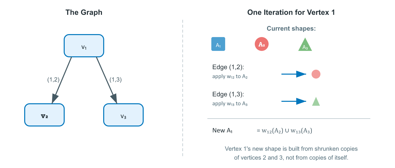
The idea is straightforward. For each vertex, look at all the edges leaving it. Each of those edges points to some other vertex and carries a contraction mapping. Apply each contraction to the target vertex's current shape, producing a shrunken copy, then take the union of all those copies. The result is the vertex's updated shape, assembled entirely from shrunken pieces of its neighbours' shapes.
In notation: for vertex $i$, the edges in $E_i$ are those with tail $i$, that is, edges whose source is $i$. Each such edge $e$ points to another vertex $e^+$, called its head, and has an associated contraction mapping $f_e$ that shrinks the head vertex's shape into a piece of vertex $i$'s shape. The GIFS operator $\mathbf{F}$ maps $n$-tuples of compact sets to $n$-tuples of compact sets, with the $i$-th component given by:
$$F_i(\mathbf{A}) = \bigcup_{e \in E_i} f_e(A_{e^+})$$
Each $f_e$ acts on $A_{e^+}$, the set at the edge's head. The contraction pulls from the head vertex back into the tail vertex $i$.
In plain language: vertex $i$'s new shape is built by taking shrunken copies of its out-neighbours' shapes and combining them. The edges determine which neighbours contribute and how. This is one complete iteration of the GIFS.
The diagram below traces through a single iteration for a three-vertex GIFS. Focus on vertex 1 to see how its new shape is assembled:
Compare this to the standard Hutchinson operator[4] $W(A) = \bigcup_{i=1}^N w_i(A)$. In the standard case, every function acts on the same set $A$. In the GIFS case, each edge acts on the specific set associated with its target vertex. The graph adds selectivity: not every component contributes to every other.
The Attractor
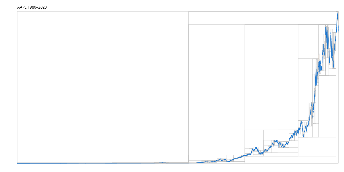
Before the formal statement, consider what the attractor means in concrete terms. Think of a rooted GIFS representing Apple's historical stock price (AAPL). The root vertex represents the entire price history, i.e., the complete pattern from IPO to today. Its outgoing edges decompose that history into, say, two major trend segments: a long secular bull run and a consolidation period. Each of those is itself a vertex in the graph, representing its own distinct pattern. Those vertices have their own edges, breaking each trend into finer sub-patterns, such as rallies, pullbacks, sideways ranges, and so on down to the leaves, which are the raw data segments.
Below is a rendering of a GIFS constructed from Apple (AAPL) stock price data where bounding boxes represent vertices at different levels.
The following is the equivalent for GSK plc (GSK), a British multinational pharmaceutical and biotechnology company. There are practical applications in using a GIFS constructed from time series data as a form of compression where key features (such as trend reversals) are preserved.
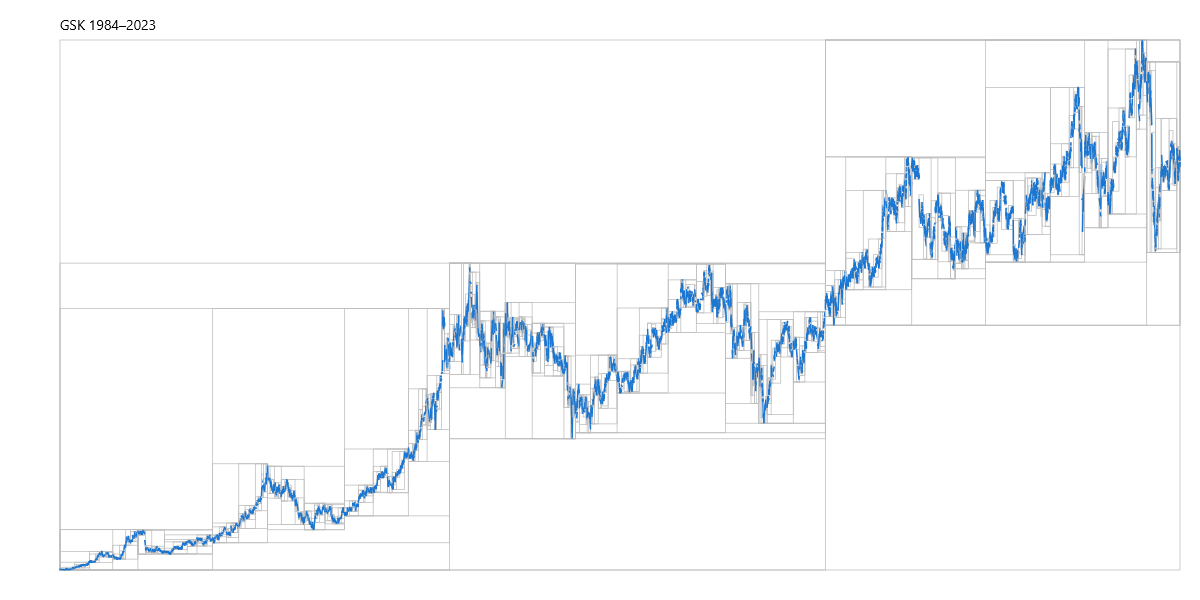
In the above pictures, every vertex in the graph is a pattern. Not a single data point or an abstract label, but a specific shape, a compact subset of time-versus-price space. The root's pattern is the whole series. An internal vertex's pattern is a segment at some level of detail. A leaf's pattern is the finest-grained piece of raw data. If you stored this graph in a database, each vertex's payload would be its pattern: the shape that the GIFS associates with that node.
The attractor is what makes this precise. Each vertex's attractor $A_i^{\ast}$ is the pattern that vertex represents, the unique shape you get when you start from a unit band (or any initial shape) at the root and apply the contraction mappings along every edge, level by level, until the result stabilises or transformation is exhausted at leaf vertices having no outgoing edges. Apply the root's edge contractions to its children's patterns, and you recover the root's pattern exactly. The attractor is the fixed point of that process: the set of patterns, one per vertex, that perfectly reproduces itself under the graph's contractions.
Just as a standard IFS converges to a single attractor shape, a GIFS converges to a tuple of attractor shapes, one for each vertex.
Start with any collection of $n$ compact shapes, one per vertex. Apply the GIFS Hutchinson operator. Each shape gets replaced by shrunken copies of its neighbours. Apply it again. And again. No matter what shapes you started with, the iteration converges to a unique fixed point: a tuple of shapes $(A_1^{\ast}, A_2^{\ast}, \ldots, A_n^{\ast})$ that reproduces itself under the operator.
Formally, the operator $\mathbf{F}$ has a unique fixed point:
$$\mathbf{F}(\mathbf{A}^{\ast}) = \mathbf{A}^{\ast}$$
This tuple $\mathbf{A}^{\ast} = (A_1^{\ast}, A_2^{\ast}, \ldots, A_n^{\ast})$ is the GIFS attractor (also called the invariant list in Edgar's terminology). Each component $A_i^{\ast}$ is a compact subset of $\mathbb{R}^d$, and each one satisfies its own self-similarity equation:
$$A_i^{\ast} = \bigcup_{e \in E_i} f_e(A_{e^+}^{\ast})$$
What this says is: each component is the union of shrunken copies of its out-neighbours' attractors. Component $A_i^{\ast}$ is built from pieces of whichever components the graph says it should be built from, not necessarily from copies of itself.
This is the crucial difference from standard IFS. In a standard IFS, the attractor is self-similar: every piece is a copy of the whole. In a GIFS, the attractor is graph-similar: each piece is a copy of whichever components the graph edges point to. This enables structures where different regions have genuinely different patterns.
Convergence. For the attractor of a general (strongly connected) GIFS to exist and be unique, the system needs to be contractive: every contraction factor must satisfy $\lambda_e < 1$, or more generally, the product of contraction factors along every closed loop in the graph must be less than 1. This ensures the Hutchinson operator is a contraction on the product hyperspace, and Banach's theorem applies. In the rooted case, the tree has no closed loops, and uniqueness follows from the tree structure and boundary data rather than from iteration, so the condition on loop products is vacuously satisfied. This is sufficient. The proof applies the Banach contraction mapping theorem to the product space $\mathbb{H}^n$, where $\mathbb{H}$ is the hyperspace of non-empty compact subsets of $\mathbb{R}^d$ equipped with the Hausdorff metric.
Theorem (Edgar, 1990; generalizing Mauldin & Williams, 1988): For any contractive GIFS, there exists a unique invariant list $(A_1^{\ast}, \ldots, A_n^{\ast})$ of non-empty compact sets, and iteration from any starting tuple converges to it.
The convergence works exactly as in the standard case:
$$d_H(\mathbf{F}^k(\mathbf{A}^0), \mathbf{A}^{\ast}) \leq \lambda^k \cdot d_H(\mathbf{A}^0, \mathbf{A}^{\ast})$$
where $\lambda = \max_e \lambda_e$ is the maximum contraction factor and $d_H$ on tuples is the maximum Hausdorff distance over components. The same geometric convergence rate, the same compound-interest-in-reverse behaviour from the IFS article.
Uniqueness in a rooted GIFS. In the classical setting above, the unique fixed point emerges from iteration: start from any shapes, apply the operator repeatedly, and the contractions force convergence to a single answer regardless of where you began. In a rooted GIFS with data-pinned leaves, uniqueness arises in a more direct way. The leaf vertices have no outgoing edges, so their attractors are not computed; they are the raw data itself. Each internal vertex's attractor is then fully determined by applying its edge contractions to its children's attractors. There is no iteration and no choice: each vertex's pattern is uniquely fixed by the data below it.
A rooted GIFS has two natural directions of use, and it helps to name them.
Construction is the bottom-up process of building a GIFS from raw data. A segmentation algorithm decomposes the time series into non-overlapping segments. These become the leaf vertices. The algorithm then groups adjacent leaves into parent segments, fits a contraction mapping to each parent-child edge that describes how the parent's shape relates to the child's, and repeats this grouping level by level until a single root vertex spans the entire series. The output is the triple $(G, \mathbf{F}, r)$: the tree, the fitted contractions, and the root. This is the harder direction, as it requires choosing where to segment, how many levels to build, and how to fit each contraction.
Rendering is the top-down process of reproducing the data from a GIFS that has already been constructed. Start with a unit bounding box at the root vertex. Apply the root's edge contractions to produce a smaller bounding box for each child. Apply each child's contractions in turn, subdividing further, and continue down through the tree until you reach the leaves. At the leaves, the contractions have mapped the original unit bounds into the precise position and scale of each data segment. The full time series is the union of these leaf-level images, and the GIFS has been rendered back into data.
Construction goes from data to GIFS; rendering goes from GIFS to data. If the contractions were fitted perfectly during construction, rendering reproduces the original series exactly. In practice, the fit is approximate, and the difference between the rendered output and the original data is the reconstruction error of the GIFS representation.
This might seem like a lesser kind of uniqueness than the classical fixed point, as it is determined by boundary conditions rather than by the deep topological argument of Banach's theorem. But the contraction property still plays an essential role. Because each edge mapping is a contraction, small perturbations in the leaf data (measurement noise, rounding, slightly different segmentation boundaries) produce bounded, smaller perturbations in the internal vertex attractors. The contractions don't just determine the answer; they stabilise it. The hierarchical structure is robust to noise in exactly the way you would want a data representation to be.
Note that for the rooted GIFS, the contraction condition can be stated more concretely than in the classical definition. What is needed is that each edge mapping strictly reduces the bounding region of its input, for instance, that the bounding box of the child's attractor is strictly contained within the bounding box of the parent's. This is weaker than pointwise Lipschitz contractivity, which requires $|f_e(x) - f_e(y)| \leq \lambda |x - y|$ for every pair of points. The pointwise condition is essential for the Banach fixed-point argument in the strongly-connected case, where convergence must be proved. In the rooted case, there is nothing to converge in that each vertex is computed once and bounding-region contractivity provides the stability that is actually needed. The next article in this series will introduce a specific parameterised transform that satisfies this bounding-region condition.
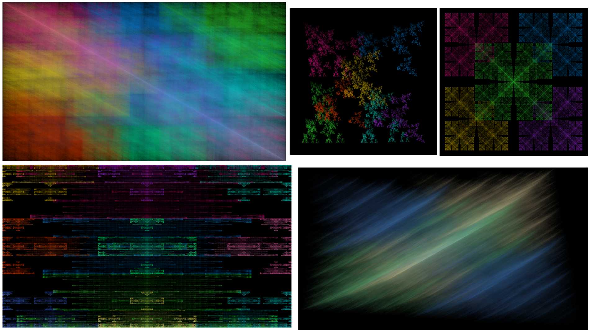
The same construction and rendering uses of GIFS can be applied to 2D images and 3D objects as well. For rendering, my GIFS implementation is capable of producing interesting images with only trivial extensions to what is used to generate time series (line charts). Reverse construction of a GIFS from an image or 3D mesh object is an area of future research, but in principle, the same segmentation and construction approach that is currently used to construct a GIFS from time series data could also be extended for images and 3D objects.
The role of strong connectivity. The classical GIFS definition requires the graph to be strongly connected, following Mauldin and Williams[5] and Barnsley and Vince[2:2]. This is not necessary for the attractor to exist (the Banach fixed point argument works for any contractive system), but strong connectivity is needed for the deeper results. Mauldin and Williams showed it is required for the Hausdorff dimension formula: the dimension $\alpha$ is the unique positive solution to $\rho([{\textstyle\sum_{e \in E_{ij}}} \lambda_e^{\alpha}]_{i,j}) = 1$, where $E_{ij}$ is the set of edges from vertex $i$ to vertex $j$ and $\rho$ denotes the spectral radius. This requires the Perron-Frobenius theorem and hence an irreducible (strongly connected) incidence matrix. Strong connectivity also ensures all attractor components are genuinely interdependent, not merely independent sub-systems living in the same graph.
Directed Self-Similarity
The most important property that distinguishes a GIFS from a standard IFS is directed self-similarity.
In a standard IFS, self-similarity is uniform: the whole attractor is the union of shrunken copies of itself. Every part looks like every other part. In a GIFS, self-similarity follows the graph structure. Component $A_i^{\ast}$ may only be similar to specific other components $A_j^{\ast}$, as determined by which edges leave vertex $i$.
This has three practical consequences.
Hierarchical structure. The graph naturally encodes parent-child relationships through edge directions. A vertex with edges pointing to several other vertices acts like a parent whose shape is composed of its children's shapes. Multi-level decompositions arise from the depth of the graph, and asymmetric dependencies, where component $A_1$ depends on $A_2$ but not vice versa, are straightforward to express.
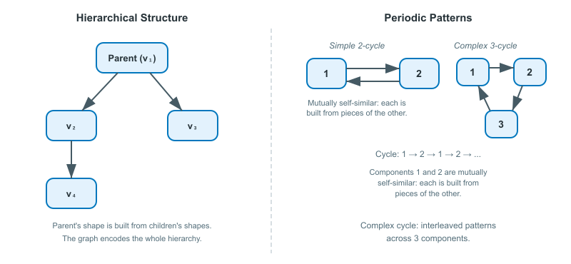
Periodic patterns. Cycles in the graph correspond to repeating motifs in the attractor. A simple cycle between two vertices means those two components are mutually self-similar: each is built from pieces of the other. More complex cycle structures produce interleaved patterns.
Controlled composition. The graph acts as a grammar for the system. Just as a grammar controls which words can follow which in a language, the GIFS graph controls which transformations can compose. This is exactly the kind of structure needed to model data with internal rules, such as the temporal ordering in a time series or the nesting in a hierarchical decomposition.
Examples
A Symmetric Network
The simplest GIFS has two vertices, $L$ and $R$, with edges connecting every vertex to every other (including self-loops). Assign contraction mappings that each shrink by half:
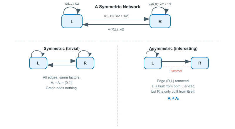
- $f_{(L,L)}(x) = \frac{x}{2}$
- $f_{(L,R)}(x) = \frac{x}{2} + \frac{1}{2}$
- $f_{(R,L)}(x) = \frac{x}{2}$
- $f_{(R,R)}(x) = \frac{x}{2} + \frac{1}{2}$
Since every vertex connects to every other vertex with identical transformations, both attractor components end up the same: $A_L^{\ast} = A_R^{\ast} = [0, 1]$. This is the GIFS equivalent of a trivial IFS. The graph structure adds nothing here because the connections are completely symmetric.
The example becomes interesting when you break the symmetry. Remove an edge, change a contraction factor, or add a third vertex with different connections, and the graph structure starts producing attractors that a standard IFS cannot.
Sierpinski Triangle with Directed Colouring
Take the Sierpinski triangle and assign each of the three half-scale copies a colour: red, green, blue. Now, instead of three interchangeable functions, build a GIFS with three vertices (one per colour) and edges that determine which colour regions map to which. For instance, with edges Red $\to$ Green, Red $\to$ Blue, Green $\to$ Red, Green $\to$ Blue, Blue $\to$ Red, and Blue $\to$ Green, but no self-loops. Each vertex's attractor is built entirely from shrunken copies of the other two colours.
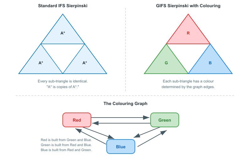
The graph controls the colouring scheme. If vertex "red" has edges pointing to "green" and "blue" but not to itself, then the red component is built from shrunken copies of the green and blue components, never from copies of itself. The overall shape is still the Sierpinski triangle, but the colouring has a structure that a standard IFS cannot express: different regions of the fractal are built from different types of sub-regions, governed by the graph.
This illustrates the core value of a GIFS. The geometry might be the same, but the relationships between parts are richer and more controlled.
GIFS Compared to Standard IFS
| Feature | IFS | GIFS (classical) | Rooted GIFS |
|---|---|---|---|
| Graph | Single vertex, self-loops | Strongly connected digraph | Rooted tree |
| Attractor | Single compact set | Tuple of compact sets | Tuple, computed bottom-up |
| Self-similarity | Uniform | Graph-directed | Hierarchical (parent-child) |
| Contraction | Pointwise Lipschitz | Pointwise Lipschitz | Bounding-region |
| Uniqueness | Banach fixed point | Banach fixed point | Tree structure + leaf data |
| Iteration required | Yes | Yes | No |
A standard IFS is a GIFS with one vertex and $N$ self-loops. Everything in the IFS article is a special case of what we've covered here.
Historical Note
Graph Iterated Function Systems were introduced by R. Daniel Mauldin and S. C. Williams in their 1988 paper "Hausdorff dimension in graph directed constructions,"[5:1] where they called the construction a graph directed construction governed by a directed graph with similarity ratios on its edges. The framework is sometimes called a Mauldin-Williams graph, particularly in Edgar's textbook[3:1] treatment and in the operator algebra literature. Other common names include graph-directed IFS, directed-graph IFS, and digraph IFS; the concept is the same across all of these, and we follow Barnsley and Vince[2:3] in using the acronym GIFS.
Elsewhere in the literature, G. C. Boore and K. J. Falconer[6] use the term DGIFS and describe the mathematics of a GIFS and a standard (1-vertex) IFS. G. C. Boore[7] has also used GIFSs to generate fractal artwork, demonstrating visually what the theory predicts: that multi-vertex directed graphs produce attractors with a richness that standard IFS cannot achieve. His gallery includes pieces built from 4-vertex systems whose components resemble variations of familiar fractals like the Sierpinski triangle, but with altered symmetry and structure in each component, a direct consequence of graph-directed self-similarity. He has also produced 4K fractal animations set to piano compositions, rendering the iterative convergence process as a visual experience on YouTube.
The original motivation was fractal geometry: computing the Hausdorff dimension of sets with non-uniform self-similarity. But the framework turned out to be far more general. GIFS became an important tool in symbolic dynamics (where the graph structure corresponds to a shift space), wavelet theory (where multiresolution analysis has a natural graph-directed interpretation), procedural modelling in computer graphics, and even aperiodic tilings of the plane. Mauldin and Urbanski later extended the framework to infinite graphs and Markov systems.
Why GIFS Matters Beyond Fractals
The step from IFS to GIFS might seem incremental, but it's the step that makes the theory applicable to structured, real-world data.
Procedural generation. In computer graphics, GIFS enables graph-directed rules for generating complex structures: cities with different building types following zoning rules, forests where tree species interact, textures with multi-scale patterns that vary across regions. The graph acts as a design grammar.
Hierarchical time series. In this article series, GIFS is the mathematical framework for representing hierarchical time series data. The vertices are types of time series segments, and the edges are the contraction mappings that relate parent segments to their children. The graph structure encodes which types of segments can contain which other types, and the attractor is the full decomposition of the series.
Symbolic dynamics. Every point in a GIFS attractor can be assigned an address, an infinite sequence of edges tracing a path through the graph. This address space has deep connections to symbolic dynamics and shift spaces, which we explore in the next section. For our purposes, the key consequence is that these addresses become natural candidates for embedding vectors.
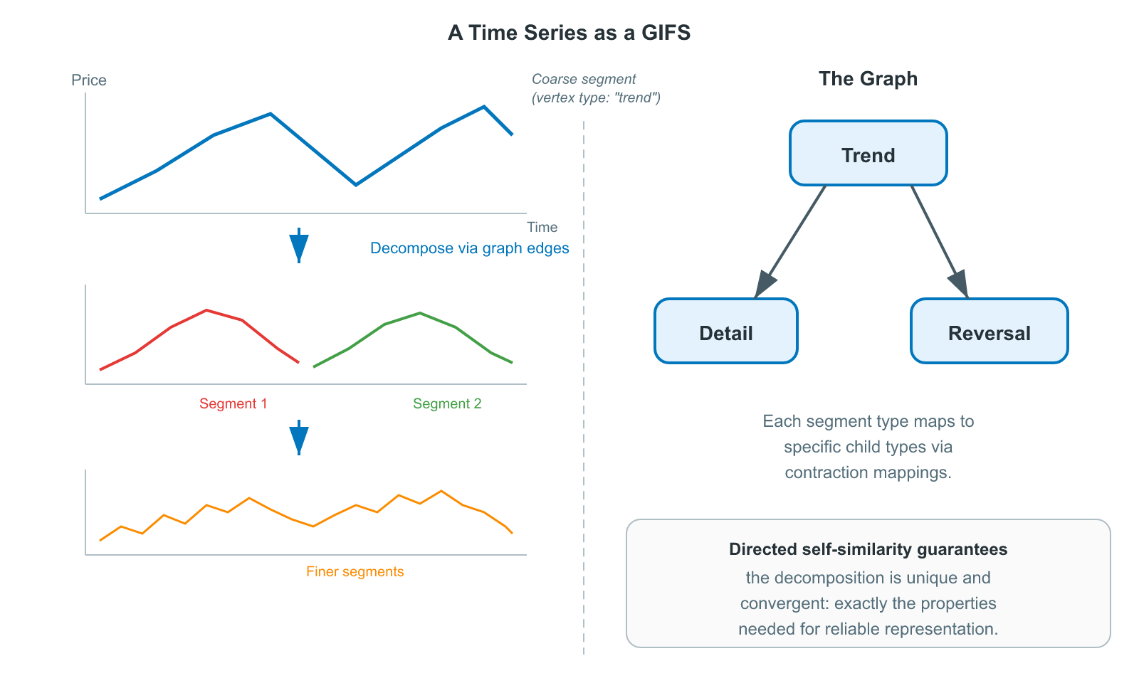
The directed self-similarity property guarantees that the decomposition is unique and convergent, exactly the properties you need for a reliable, reproducible representation.
Symbolic Dynamics: From Addresses to Embeddings
To understand why these addresses matter, we need a concept from symbolic dynamics: the shift space.
A shift space is the set of all infinite sequences you can form from a finite alphabet (here, the edge labels of the graph) subject to rules about which symbols can follow which. The "shift" refers to the operation of dropping the first symbol and sliding everything one position to the left, like reading the next chapter of a book and forgetting the first. A subshift of finite type is a shift space where the rules are determined by a finite graph: symbol $b$ can follow symbol $a$ if and only if there is an edge from $a$'s target vertex to $b$'s source vertex.
In a GIFS, the graph's adjacency matrix is exactly this rule set, i.e., it determines which contractions can compose, and therefore which infinite address sequences are valid. The set of all valid addresses forms a subshift of finite type. This establishes a deep link between fractal geometry and symbolic dynamics: the combinatorial structure of allowed paths through the graph mirrors the geometric structure of the attractor. Two addresses that share a long common prefix correspond to points that are geometrically close, because they have passed through the same sequence of contractions for many steps. The symbolic (combinatorial) notion of proximity and the geometric (metric) notion of proximity are aligned.
Addresses in a Rooted GIFS
In our data-pinned rooted GIFS, addresses become simpler and more concrete. Because the graph is a finite tree, every vertex has a unique path from the root, and that path is the vertex's address. The address is a finite sequence of edges, not an infinite one, and it encodes exactly where in the hierarchy the vertex sits: which branch was taken at the root, which sub-branch at the next level, and so on down to the leaf. Reading the address root-to-leaf gives the decomposition path, or how the whole series was subdivided to reach this particular segment. Reading it leaf-to-root gives the composition path, or how this segment assembles upward into progressively coarser patterns.
From Addresses to Embeddings
These finite addresses are natural candidates for embeddings. An embedding, in the machine learning sense, is a fixed-length numerical vector that represents a complex object (for example, a word, an image patch, or a time series segment) in a way that preserves meaningful relationships. Objects that are similar in the real world end up close together in the vector space; objects that are dissimilar end up far apart. Modern neural networks, including transformers, operate entirely on these vector representations: they don't see raw text or raw pixels, they see embeddings. Here, "transformers" refers to the architecture behind Large Language Models (LLMs) as used by AI chatbots such as ChatGPT.
A GIFS address already encodes exactly the kind of structure an embedding needs to capture. Each address records a vertex's position in the hierarchy and the sequence of contractions connecting it to every level of detail. The transformation parameters at each edge (encoding scale, position, and shape) are numerical, so each edge contributes a small vector of numbers, and the full address is a composition of these vectors from root to leaf. Two vertices that share a long common prefix (same branch of the tree for many levels) will have similar embeddings; vertices on distant branches will be far apart.
The geometry of the GIFS tree maps directly into the geometry of the embedding space, which is the high-dimensional vector space in which all these embeddings live. An embedding space is not just a set of unrelated vectors; it has structure. Directions in the space correspond to meaningful properties, and distances between vectors reflect how similar the underlying objects are. In a well-known example from natural language processing, the embedding space for words places "king" and "queen" close together and in the same direction from "man" and "woman," capturing the analogy without anyone having programmed it explicitly. The space itself learns to encode relationships.
For a GIFS, the embedding space inherits structure from the tree. Vertices at the same depth (same level of detail) occupy a similar region of the space. Siblings (children of the same parent) are nearby but distinguishable by their individual contraction parameters. The root-to-leaf path defines a trajectory through the space from coarse to fine, and the contraction parameters at each edge determine the step. The result is an embedding space where proximity means structural similarity in the hierarchical decomposition, which is exactly the kind of geometric organisation that allows a transformer to detect patterns across different segments, different scales, and different time series.
This is the bridge from the graph-theoretic structure of the GIFS to the vector spaces that a transformer operates on. The next article in this series introduces the shard transform: a concrete, parameterised edge mapping in $(0, 1)^8$ that encodes the parent-child relationship at each edge as a combination of scale, position, and shape deformation. Each edge contributes 8 numbers; a root-to-leaf path contributes $8D$ numbers; and the resulting embeddings form the input to a temporal transformer. The shard transform satisfies the bounding-region contractivity needed for the rooted GIFS while providing a parameter space where every point is a valid transform and where distance reflects structural similarity, i.e., the properties needed for vector search and for learning over hierarchical decompositions.
What's Next in This Series
This article showed how adding a directed graph to an IFS gives the theory the expressiveness needed for structured, non-uniform self-similarity. The next article will bridge from fractal geometry to machine learning, showing how the GIFS decomposition creates a vocabulary for time series and how contraction parameters become the embeddings that a temporal transformer operates on.
Previously: Iterated Function Systems · Next: Temporal Embeddings
References
Barnsley, M. F. (1988). Fractals Everywhere. Academic Press. ↩︎
Barnsley, M., Vince, A. Tilings from graph directed iterated function systems. Geom Dedicata 212, 299–324 (2021). doi.org/10.1007/s10711-020-00560-4 ↩︎ ↩︎ ↩︎ ↩︎
Edgar, G. A. (1990, 2nd ed. 2008). Measure, Topology, and Fractal Geometry. Springer. Textbook treatment of GIFS under the name "Mauldin-Williams graph." ↩︎ ↩︎
Hutchinson, J. E. (1981). "Fractals and self-similarity". Indiana University Mathematics Journal, 30(5), 713-747. ↩︎
Mauldin, R. D., & Williams, S. C. (1988). "Hausdorff dimension in graph directed constructions". Transactions of the American Mathematical Society, 309(2), 811-829. ↩︎ ↩︎
G. C. Boore and K. J. Falconer, Attractors of directed graph IFSs that are not standard IFS attractors and their Hausdorff measure, Math. Proc. Camb. Phil. Soc. 154 (2013), 324-349. doi.org/10.1017/S0305004112000576 ↩︎
G. C. Boore, Directed Graph Iterated Function Systems, (online). directed-graph-iterated-function-systems. Accessed on Feb. 2026. ↩︎