Iterated Function Systems: The Simple Rules Behind Complex Fractals

How a handful of shrinking functions, applied over and over, can generate the infinite complexity of fractal geometry.

This article series establishes the mathematical foundations for representing time series as self-similar hierarchical structures, a framework that underpins a novel AI architecture for timeseries data. This first article covers the core mechanism: how a small set of contraction mappings, iterated to a fixed point, can encode complex structure from simple rules.

Next in this series: Graph Iterated Function Systems

Take a fern leaf. Look closely at one of its fronds, and you'll see it looks like a miniature copy of the whole leaf. Zoom into a frond of that frond, and the pattern repeats. Nature is full of this kind of structure -- coastlines, trees, blood vessels, mountain ranges -- i.e., shapes that echo themselves at different scales.

In 1981, a mathematician named John Hutchinson showed that you can capture this self-repeating structure with a remarkably simple recipe: take a small collection of functions, each of which shrinks and repositions a shape, and apply them over and over. No matter what shape you start with, this process always converges to the same intricate pattern, a fractal. The fractal is entirely determined by the rules, not by the starting shape.

This recipe is called an Iterated Function System, or IFS. It's one of the most elegant ideas in mathematics, and it turns out to be far more than a curiosity. IFS underpins fractal image compression, procedural generation in computer graphics, and, as I'll hint at the end, new ways of thinking about time series data. If you've ever wondered how a few simple rules can produce infinite complexity, this is the article for you.

We'll build up the theory step by step, with both the intuition and the formal mathematics. You don't need to be a mathematician to follow along, but I won't shy away from the formulas. They're what make the ideas precise.

Why "Iterated"?

The word iterated is the key to understanding what an IFS does. An IFS is not merely a collection of functions. It is a recipe for applying them over and over again.

Start with any shape: a square, a circle, a single point -- it doesn't matter. Apply every function in the system to that shape, collect the results, and you have a new shape. Now do it again. And again. Each round of application is one iteration. With each iteration the shape gets closer to the system's attractor, i.e., a fixed fractal pattern that doesn't change when you apply the functions one more time.

This repeated application is exactly what makes the system iterated: the output of one round becomes the input to the next. The remarkable property is that no matter what shape you start with, the iteration always converges to the same attractor. The starting shape is forgotten; only the functions themselves determine the final result.

To make this concrete, suppose you define two functions that each shrink and shift a shape (we'll see the Cantor set example later). Then:

• Iteration 0: Start with the unit interval [0, 1].
• Iteration 1: Apply both functions and you get two shorter segments.
• Iteration 2: Apply both functions to each segment and you get four even shorter segments.
• Iteration 3: Eight segments, and so on...

After infinitely many iterations, you arrive at the Cantor set. It is this process of feeding results back through the same functions that earns the name "iterated".

With that intuition in place, let's pin down exactly what an IFS is.

Definition

At its core, an IFS is just a short list of functions that all share one property: each one makes things smaller. You pick a space to work in (a line, a plane, or any setting where you can measure distance), and you define a handful of functions that shrink and reposition points within that space. The "shrinking" requirement is what guarantees the iteration converges instead of spiraling out of control. Think of each function as a photocopier that produces a reduced, shifted copy of whatever you feed it.

An Iterated Function System consists of two components:

1. A complete metric space $(X, d)$ as the "canvas" on which everything takes place. For example, the real number line, or the 2D plane with the usual notion of distance.
2. A finite set of contraction mappings ${w_1, w_2, \ldots, w_N}$ as a set of functions that each squeeze space closer together. Each $w_i: X \to X$ has a contraction factor $s_i < 1$, meaning it reduces distances by at least that factor.

Written as a tuple (an ordered collection of elements bundled together) an IFS is:

$$\mathcal{W} = (X, {w_1, w_2, \ldots, w_N})$$

That's it. A space and a list of shrinking functions. The contraction requirement means that for any two points $x$ and $y$:

$$d(w_i(x), w_i(y)) \leq s_i \cdot d(x, y)$$

In plain language: after applying $w_i$, any two points end up strictly closer together than they were before. This is the crucial constraint. Because every function shrinks distances, the iteration can't blow up. It has to settle down. The strength of the contraction (how small $s_i$ is) determines how quickly it settle. See the books by Barnsley^[1], Falconer^[2], Peitgen et al^[3] and Edgar^[4] for detailed descriptions of standard IFSs.

Now that we have the ingredients, we need a way to describe what happens when we apply all the functions at once. That's where the Hutchinson operator comes in.

The Hutchinson Operator

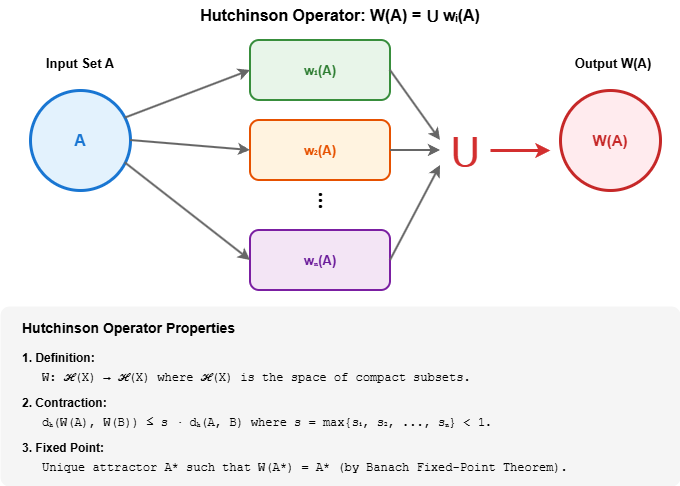
When running an IFS by hand, you would take your current shape, feed it through every function in the system, and then overlay all the shrunken copies to form a new shape. The Hutchinson operator is simply the name for doing all of that in one step. It is the "iterate once" button: give it a shape, and it hands back the next shape in the sequence.

Given a compact set $A$ (think of it as a shape in the space), the Hutchinson operator $W$ produces a new set by applying every function to $A$ and taking their union:

$$W(A) = \bigcup_{i=1}^N w_i(A) = w_1(A) \cup w_2(A) \cup \cdots \cup w_N(A)$$

Each $w_i(A)$ is a shrunken, repositioned copy of $A$. The union collects all of them into one new shape. This is one complete iteration.

Here's the key theorem that makes the whole theory work:

Theorem (Hutchinson, 1981): Because each $w_i$ is a contraction, the Hutchinson operator itself is a contraction on the space of compact subsets, equipped with the Hausdorff metric $d_H$:

$$d_H(W(A), W(B)) \leq s \cdot d_H(A, B)$$

where $s = \max{s_1, s_2, \ldots, s_N} < 1$.

What this means is: take any two shapes $A$ and $B$, no matter how different they look. Apply the Hutchinson operator to both. The resulting shapes $W(A)$ and $W(B)$ are guaranteed to be more similar to each other than $A$ and $B$ were. The operator brings any two shapes closer together, by at least the factor $s$, every single time it is applied. This is the engine that drives convergence.

And since the Hutchinson operator is itself a contraction, we can invoke one of the most powerful results in mathematics to guarantee that the iteration has a destination. That destination is the attractor.

The Attractor

If you keep pressing the "iterate" button, the shapes you produce settle down to a single, stable pattern. This is the attractor which is the fractal that the IFS is "trying to draw".

The attractor has a remarkable property: applying the IFS functions to it produces exactly itself. It is a fixed point of the process, and it is the only one. No matter what shape you started with -- a dot, a square, a squiggle -- the iteration forgets the starting shape and converges to the same attractor. The attractor is determined entirely by the functions, not by the initial conditions.

Since the Hutchinson operator is a contraction, the Banach Fixed-Point Theorem guarantees it has a unique fixed point $A^{\ast}$:

$$W(A^{\ast}) = A^{\ast}$$

This equation says: apply all the IFS functions to $A^{\ast}$ and take the union, and you get $A^{\ast}$ back unchanged. The shape reproduces itself under its own rules. This fixed point is the attractor.

Convergence from any starting point. Pick any compact set $A_0$ as a starting shape and define the iteration:

$$A_{n+1} = W(A_n) = \bigcup_{i=1}^N w_i(A_n)$$

Then $A_n$ converges to $A^{\ast}$ in the Hausdorff metric:

$$\lim_{n \to \infty} d_H(A_n, A^{\ast}) = 0$$

The convergence is geometric at rate $s^n$. Think of it like compound interest running in reverse: after each iteration, the remaining distance to the attractor is multiplied by $s$ (which is less than 1). After $n$ iterations, the error is at most $s^n$ times the initial distance. When $s$ is small (a strong contraction) you get there fast. When $s$ is close to 1, convergence is slow but still guaranteed.

Three Properties That Make IFS Powerful

The attractor of an IFS has three properties that together make the theory so useful.

Self-Similarity. The attractor equation $A^{\ast} = \bigcup_{i=1}^N w_i(A^{\ast})$ says that the attractor is the union of $N$ contracted copies of itself. Zoom into any piece produced by one of the $w_i$, and you see the whole attractor again. This is the formal definition of self-similarity.

Invariance. The attractor is invariant under the Hutchinson operator: applying the IFS transformations reproduces the same set. It is the shape that "survives" the iteration unchanged.

Uniqueness. The attractor is the unique non-empty compact set satisfying the self-similarity equation. No matter what initial set $A_0$ you choose, e.g., a single point, a filled square, an arbitrary blob, the iteration always converges to the same $A^{\ast}$. The functions alone determine the fractal.

Together, self-similarity, invariance, and uniqueness mean that an IFS is a compact description of a potentially infinitely complex shape. A handful of numbers (the parameters of a few contraction mappings) fully determines a fractal. This is what makes IFS so attractive for compression, generation, and analysis.

Examples

The best way to understand an IFS is to see it in action. The three examples below range from the simplest possible fractal to a surprisingly realistic natural form. In each case, a small number of simple rules produces an intricate structure through nothing more than repetition.

The Cantor Set: Fractal Dust from Two Rules

The Cantor set is the simplest IFS that produces a non-trivial fractal. Start with the unit interval, i.e., the line segment from 0 to 1. Two functions each keep a third of the segment and discard the middle, then repeat. After infinitely many repetitions, what remains is a dust of points: uncountably many, yet with zero total length.

The IFS operates on $[0, 1]$ with two functions:

$$w_1(x) = \frac{x}{3}, \quad w_2(x) = \frac{x}{3} + \frac{2}{3}$$

Both functions shrink by a factor of 3 ($s = 1/3$). $w_1$ maps into the left third of the interval, $w_2$ into the right third. The middle third is never covered, and it is this gap, repeated at every scale through iteration, that produces the Cantor set.

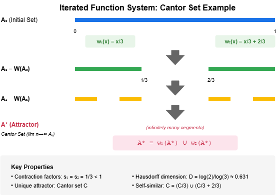
Walking through the iteration:

• Start: $A_0 = [0, 1]$
• After 1 iteration: $A_1 = [0, 1/3] \cup [2/3, 1]$ (middle third removed)
• After 2 iterations: $A_2 = [0, 1/9] \cup [2/9, 1/3] \cup [2/3, 7/9] \cup [8/9, 1]$
• In the limit: The Cantor set -- uncountably many points, yet with total length zero.

If you want to build an intuition for this, try it with a pencil and a ruler. Draw a line. Erase the middle third. Now erase the middle third of each remaining segment. By the third or fourth round, the pattern is unmistakable, and you've just run an IFS by hand.

The Sierpinski Triangle: Self-Similarity in Two Dimensions

Moving from lines to the plane, the Sierpinski triangle shows IFS generating a two-dimensional fractal. Take any filled triangle and replace it with three half-sized copies, one at each corner. The centre is always left empty. Repeat, and a lace-like pattern emerges: a shape built entirely from smaller versions of itself.

The IFS uses three contractions on $\mathbb{R}^2$, each scaling by $\frac{1}{2}$ toward one vertex:

$$w_1(x, y) = \frac{1}{2}(x, y), \quad w_2(x, y) = \frac{1}{2}(x, y) + \left(\frac{1}{2}, 0\right), \quad w_3(x, y) = \frac{1}{2}(x, y) + \left(\frac{1}{4}, \frac{\sqrt{3}}{4}\right)$$

Each iteration replaces the current shape with three half-sized copies, one at each corner. The centre triangle is always empty. The attractor is the Sierpinski triangle, a shape that contains three copies of itself, each at half scale.

There's a beautiful party trick related to this fractal called the chaos game. Pick three points as the vertices of a triangle. Now pick any random starting point. Repeatedly choose one of the three vertices at random, and move halfway toward it. Plot each new point. Despite the randomness, after a few hundred points, the Sierpinski triangle appears as if by magic. This works because every function in the system is a contraction -- no matter which vertex is chosen, the point is pulled toward the attractor. Over many iterations, the point visits every part of it.

The Barnsley Fern: Nature Encoded in Four Rules

The Barnsley fern is the example that makes most people sit up and pay attention. Four functions, each a simple affine transformation (scale, rotate, shift), are enough to generate a fern that is strikingly realistic. That's worth pausing on: the entire structure of a fern leaf, with its stem, its fronds, and the fronds of its fronds, is encoded in just four rules and a handful of numbers.

Here's how the four functions divide the work:

• $w_1$ maps everything to the stem, i.e., a thin line along the base (chosen with probability 0.01).
• $w_2$ copies the entire fern, slightly smaller and rotated, to create a leaflet on the right.
• $w_3$ does the same on the left.
• $w_4$ stretches the fern upward, creating the main body.

The probabilities control the visual density: the stem function fires rarely (it's just a thin line), while the leaflet and body functions fire frequently, filling out the fern's structure. The attractor is the fern, i.e., a demonstration that a handful of simple contraction mappings, iterated, can encode complex natural structure.

This is the power of IFS distilled to a single image: nature's complexity emerging from mathematical simplicity.

The Collage Theorem: Working Backwards

So far we've gone in one direction: given functions, find the attractor. But in practice you often want to go the other way. You have a target shape (such as an image, a coastline, a dataset) and you want to find an IFS whose attractor approximates it. The Collage Theorem tells you how.

The idea is intuitive: if you can tile your target shape with shrunken, shifted copies of itself (a "collage"), and the collage is a close match, then the IFS built from those shrink-and-shift operations will produce an attractor close to the target. The better the collage, the better the approximation.

Theorem (Barnsley, 1985): If an IFS with Hutchinson operator $W$ makes a target shape $L$ look like a collage of shrunken copies of itself, that is, $W(L) \approx L$, then the attractor $A^{\ast}$ is guaranteed to be close to $L$:

$$d_H(L, A^{\ast}) \leq \frac{1}{1 - s} \cdot d_H(L, W(L))$$

In other words: minimize the collage error $d_H(L, W(L))$, and the attractor automatically becomes a good approximation. The factor $\frac{1}{1-s}$ amplifies the error, but since $s < 1$, this amplification is finite, and for strong contractions it's modest.

This theorem is what makes IFS practically useful. Instead of storing a complex shape point by point, you can search for a small set of contraction mappings whose collage matches the shape. Store those few parameters, and the IFS will reconstruct the shape to any desired resolution. This is the theoretical basis of fractal compression, which we'll touch on below.

Fractal Dimension

Everyday objects have integer dimensions: a line is 1-dimensional, a filled square is 2-dimensional. Fractals break this rule. The Cantor set is too spread out to be a single point (dimension 0) but too sparse to be a line (dimension 1), i.e., it lives somewhere in between. The Sierpinski triangle is more than a line but less than a filled region. This "in-between" dimension is called the Hausdorff dimension, and it measures how thoroughly a fractal fills the space around it.

For self-similar IFS where all $N$ functions have the same contraction factor $s$, the dimension has an elegant closed-form expression. It satisfies:

$$N \cdot s^D = 1 \implies D = \frac{\log N}{\log(1/s)}$$

The intuition: $N$ copies at scale $s$ must tile the attractor perfectly. The dimension $D$ is the exponent that balances the number of copies against how much each one is shrunk. More copies or less shrinking means a higher dimension (the fractal fills more space); fewer copies or more shrinking means a lower dimension (the fractal is sparser).

Examples:

• Cantor set: $N=2$ copies, each at scale $s=1/3$ gives $D = \frac{\log 2}{\log 3} \approx 0.631$ somewhere between a point and a line.
• Sierpinski triangle: $N=3$ copies, each at scale $s=1/2$ gives $D = \frac{\log 3}{\log 2} \approx 1.585$ somewhere between a line and a filled triangle.

Historical Note

The theory of Iterated Function Systems was formalized by John Hutchinson in his 1981 paper "Fractals and self-similarity", which established the mathematical foundations: the contraction mapping framework, the Hutchinson operator, and the existence and uniqueness of attractors. Michael Barnsley then popularized IFS in the late 1980s, particularly through his book Fractals Everywhere (1988), which demonstrated IFS as a practical tool for fractal generation and introduced the Collage Theorem as the basis for fractal image compression.

The key insight they established: self-similar structures can be compactly represented as the attractor of a small set of contraction mappings. This idea has influenced fields from computer graphics to data compression, and, as we'll see in this series, it extends naturally to the analysis of temporal data and timeseries.

Why IFS Matters Beyond Fractals

IFS started as a way to formalize fractal geometry, but its reach extends well beyond pretty pictures.

Fractal image compression. In the early 1990s, Arnaud Jacquin showed that real photographs contain enough approximate self-similarity to be compressed using IFS. Instead of storing pixel values, you store the contraction mappings that reconstruct the image. The compression ratios were impressive, and while wavelet-based methods eventually won out for general image compression, the IFS approach demonstrated something profound: real-world data has self-similar structure that compact mathematical descriptions can exploit.

Computer graphics and procedural generation. Game engines and film studios used IFS-like systems to generate realistic landscapes, vegetation, and textures. The Barnsley fern is just the beginning. The same principle of iterating simple rules to produce complex forms drives much of procedural content generation.

Time series and hierarchical data. In my own research, I'm exploring extensions of IFS that represent hierarchical time series data. The core idea is that a time series can be decomposed into a hierarchy of segments, where each parent segment relates to its children through contraction mappings. The hierarchy is an IFS, and the properties we've covered, such as convergence, uniqueness, self-similarity, translate directly into guarantees about reconstruction accuracy. But that's a story for the next article.

What's Next in This Series

This article covered the foundations: what an IFS is, why iteration converges, and how a handful of contraction mappings can encode infinitely complex structure. The next article will introduce Graph Iterated Function Systems (GIFS), a generalization where the functions are organized into a directed graph, constraining which transformations can follow which. This added structure enables richer, more controlled patterns and is the bridge between classical IFS theory and its application to real-world time series data.

If you found this useful, follow along for the rest of the series. Each article builds on the last, working toward a framework where the elegant mathematics of IFS meets the messy reality of time series analysis.

Next: Graph Iterated Function Systems

References

Barnsley, M. F. (1988). Fractals Everywhere. Academic Press. ↩︎
K. J. Falconer, Fractal Geometry, Mathematical Foundations and Applications, John Wiley, Chichester, 2nd Ed. (2003). ↩︎
H-O. Peitgen, H. Jürgens and D. Saupe, Chaos and Fractals: new frontiers of science, Springer-Verlag, New York, (2004). ↩︎
G. A. Edgar, Measure, Topology, and Fractal Geometry, Springer-Verlag, New York, 2nd Ed. (2000). ↩︎